Thursday, December 15, 2011

Plank's Constant Lab

In this experiment we were trying to measure the planks constant. The setup for the experiment is the same as light spectra setup with a few differences. First of all, the light source instead of a heated gas are 4 LEDs, blue, green, yellow and red.  Also for this experiment we used a voltage source to illuminate the LED's since those LEDs did not work with AC power. From the experiment we obtained voltage across the LEDs and also the associated wavelengths for the LEDs.


d= 2*10^-6 m = 500 slits per mm
D= distance of the light spectra 
L= 0.97 ± 0.005 m


The picture above shows both the green LED and its view through the diffraction grating.


as you can see it is really hard to point at a position with high precision for D. That is the reason we end up getting a huge uncertainty to compensate for the measurement difficulties.
Next is the table for λ and its associated voltage and the graph of voltage vs 1/λ.

                        ±0.001              ±42767

The horizontal axis on the graph is the 1/λ and the vertical is the voltage.
Using the following formula we calculated the planks constant:
where e is charge of an electron and V is the voltage measured across the LED by a meter and finally c is the speed of light.
e = 1.602E-19
c=3E8

The values calculated from measurement all agree with h within uncertainty. However the most amount of error is associated with green and yellow which as mentioned before might be due to the fact that while we were looking through the grating the least resolved and sharp light lines were from green and yellow and that is why they are both from the actual value by 7 and 10 percent respectively. 


Visualizing Wave Packets

In this lab the purpose was to get a better understanding of wave packets through computational modeling since it is not possible to do physical experiments with current equipments. So the code for the programing is as follow:


from pylab import *
w=1 
Fourier_Series=[] 
sigma = 10
C1 = 1
numberofharmonics=50
center = numberofharmonics/2

for i in range(1,50):#every time the loop repeats this will change the harmonic
    x = [] # plots from -pi to +pi
    gauss = C1*exp(-(i-center)**2/(2.*sigma**2))
    sin_list = [] #this includes the sine functions
    for t in arange (-3.14, 3.14, 0.01): 
        sine= gauss*sin(i*w*t) 
        sin_list.append(sine) 
        x.append(t)
    #plot(x,sin_list)# plots values
#show()

    Fourier_Series.append(sin_list)
superposition = zeros(len(sin_list))
for function in Fourier_Series:
    for i in range(len(function)):
        superposition[i]+=function[i]
plot(x,superposition)
show()


Answers to the questions at the end of the handout:

 1)

2)

3) L
4) 2L
5) ---- (same question as last part)
6) h
7) h
8) In both cases the values are equal to h which means the results are bounded and cannot pass this value which ties itself to uncertainty principal.

In pursuit of lambda :D

 Today after a huge nonexistence period of exciting lab experiments, we did a very helpful and exciting lab on obtaining lambdas associated with light spectrum and then identifying an unknown gas using the same principle as before and a gas spectrum table.

For all three experiments we used the following setup to find the associated wavelengths of visible light from violet to red and then the spectra for an unknown gas and at the end compare measured spectral lines of Hydrogen to actual values..
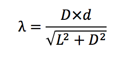
L= Distance between the diffraction grating and the light source = 2±0.02m 
the large uncertainty on L is due to the fact that the light source could not be perfectly put on the zero mark and so we moved the diffraction grating in a way to get as close as possible to 2 meters.
D= Distance to the light line seen through  the grating (in this case start of red)

λ=wavelength of the light line
d=grade of the diffraction grating= 2×10⁻⁶ m (500 slits per mm)


First Experiment : White Light Spectra
This is the light spectra of a light bulb through diffraction grating


If we compared the data from the experiment to the actual values the only ones that are not matching within the uncertainty are green and orange. The reason is before green is cyan and before and after the orange are yellow and red respectively. In both cases it was hard for both of us to differentiate exactly the beginning of the those two colors. So we should just increase the uncertainty in the measurement to about 20 nm. 
Another error corresponding to the uncertainty is the fact that the small angle approximation does not hold true in this experiment since the smallest value for it is from violet.
D=0.39 which gives an angle of 11 degrees or 0.193 rad. the sin of this angle is 0.193 which still holds true for small angle approximation but with red and D=0.7775 the angle is 0.37 rad 0.362. These differences though not big, still add to the overall uncertainty.


                          Second Experiment : Unknown Gas
The exact setup as the first experiment was implemented. The same measurements were taken and same formulas were used.


The Unknown Gas's Spectral Lines Through the Gratings


After observing the spectral lines and obtaining wavelengths values we compared these values with given other gases' spectral line we concluded that the gas was Helium. Eventually it turned out that the gas was Mercury. 


The one before last spectra is Mercury and the one before that is Helium. From this picture it is obvious why we confused the two together.


the smaller uncertainty on this experiment for D is because we took the measurements more carefully and with more trials.


This graph is a graph of the linear relationship between the actual wavelength to calculated one. This equation for the graph acts as a linear adjustment that compensates for systematic error and any faulty steps. 


with the new linear adjustment the error becomes less than 1%.


Third Experiment : 
Third experiment is the repeat of second one, however in this one the gas is known which is Hydrogen. The goal is to compare our measured values to actual values and see if our linear adjustment is still a true adjustment. 


The uncertainty on the adjusted wavelengths is the same as primary calculated wavelength since the transformation is linear that number does not change.
After comparing the values it is proven that firstly this gas is truly Hydrogen and secondly our linear adjustment is a total error annihilator.

Wednesday, December 14, 2011

Active Physics 2

Electron Trap: Particle in a Box
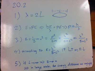
The following pictures are the answers to problem s from section 20.2 of Pearson's Active Physics.
http://wps.aw.com/aw_young_physics_11/13/3510/898597.cw/index.html


Tuesday, December 13, 2011

Active Physics

These are pictures of the answers to 17.1 and 17.2 from the Pearson's Active Physics.
http://wps.aw.com/aw_young_physics_11/13/3510/898597.cw/index.html


17.1


17.2

Measuring CD Track Spacing

In this lab the goal was to find the spacing of tracks of a regular CD. To do so we used a laser and we pointed it at the CD and the reflection was observed on a whiteboard. The setup was as follow:

The result from this setup looked like this:


Even though the dots are clear the curving in the pattern makes the geometry harder. The curving happens due to the fact that the CD is round, so a CD grating is different compare to the regular gratings used in class. For this reason we changed our setup in following manner:


This way the diffraction pattern would not curve as much and everything can easily be measured with a meter stick.


The formula for the diffraction is:


where θ is the angle between zeroth maxima to the first maxima, λ is the wavelength of the red laser, m is the number of the maxima and d is the grating which is what we were looking for.

y=27±0.5cm
λ=650±20nm


x= m=17±1cm
m=1


since this value equals 32.2 degrees we cannot use small angle approximation. After plugging in the proper values the value obtained for spacing is 1220

which equals 1220±0.5 μm


however the value given for a track spacing is about 1600 μm. If we take into account the uncertainty maximum value for the spacing with our value is 1332 μm which is still off by about 16% from 1600 μm
this shows that there is error somewhere in the experiment that we hav'nt accommodated for, or the geometry and setup of the experiment is faulty.

Thursday, October 20, 2011

VPython Code

To get some practice in class with programing and specificallyVPython, Brian and I had to do exercise number 5 of the second handout.
So here is the code and the result:


from math import *


A=zeros(100,float)
B=zeros(100,float)
C=zeros(100,float)
Sum=0
D=float


for i in range(0,100):
    A[i]= sin(2*pi*i/100)
    B[i]= cos(2*pi*i/100)
    C[i]=A[i]*B[i]
for i in range(0,100):
    D=Sum+C[i]
    Sum=D
    
        
print A
print B
print C
print "sum of all values is", Sum 


[  0.00000000e+00   6.27905195e-02   1.25333234e-01   1.87381315e-01
   2.48689887e-01   3.09016994e-01   3.68124553e-01   4.25779292e-01
   4.81753674e-01   5.35826795e-01   5.87785252e-01   6.37423990e-01
   6.84547106e-01   7.28968627e-01   7.70513243e-01   8.09016994e-01
   8.44327926e-01   8.76306680e-01   9.04827052e-01   9.29776486e-01
   9.51056516e-01   9.68583161e-01   9.82287251e-01   9.92114701e-01
   9.98026728e-01   1.00000000e+00   9.98026728e-01   9.92114701e-01
   9.82287251e-01   9.68583161e-01   9.51056516e-01   9.29776486e-01
   9.04827052e-01   8.76306680e-01   8.44327926e-01   8.09016994e-01
   7.70513243e-01   7.28968627e-01   6.84547106e-01   6.37423990e-01
   5.87785252e-01   5.35826795e-01   4.81753674e-01   4.25779292e-01
   3.68124553e-01   3.09016994e-01   2.48689887e-01   1.87381315e-01
   1.25333234e-01   6.27905195e-02   1.22464680e-16  -6.27905195e-02
  -1.25333234e-01  -1.87381315e-01  -2.48689887e-01  -3.09016994e-01
  -3.68124553e-01  -4.25779292e-01  -4.81753674e-01  -5.35826795e-01
  -5.87785252e-01  -6.37423990e-01  -6.84547106e-01  -7.28968627e-01
  -7.70513243e-01  -8.09016994e-01  -8.44327926e-01  -8.76306680e-01
  -9.04827052e-01  -9.29776486e-01  -9.51056516e-01  -9.68583161e-01
  -9.82287251e-01  -9.92114701e-01  -9.98026728e-01  -1.00000000e+00
  -9.98026728e-01  -9.92114701e-01  -9.82287251e-01  -9.68583161e-01
  -9.51056516e-01  -9.29776486e-01  -9.04827052e-01  -8.76306680e-01
  -8.44327926e-01  -8.09016994e-01  -7.70513243e-01  -7.28968627e-01
  -6.84547106e-01  -6.37423990e-01  -5.87785252e-01  -5.35826795e-01
  -4.81753674e-01  -4.25779292e-01  -3.68124553e-01  -3.09016994e-01
  -2.48689887e-01  -1.87381315e-01  -1.25333234e-01  -6.27905195e-02]
[  1.00000000e+00   9.98026728e-01   9.92114701e-01   9.82287251e-01
   9.68583161e-01   9.51056516e-01   9.29776486e-01   9.04827052e-01
   8.76306680e-01   8.44327926e-01   8.09016994e-01   7.70513243e-01
   7.28968627e-01   6.84547106e-01   6.37423990e-01   5.87785252e-01
   5.35826795e-01   4.81753674e-01   4.25779292e-01   3.68124553e-01
   3.09016994e-01   2.48689887e-01   1.87381315e-01   1.25333234e-01
   6.27905195e-02   6.12323400e-17  -6.27905195e-02  -1.25333234e-01
  -1.87381315e-01  -2.48689887e-01  -3.09016994e-01  -3.68124553e-01
  -4.25779292e-01  -4.81753674e-01  -5.35826795e-01  -5.87785252e-01
  -6.37423990e-01  -6.84547106e-01  -7.28968627e-01  -7.70513243e-01
  -8.09016994e-01  -8.44327926e-01  -8.76306680e-01  -9.04827052e-01
  -9.29776486e-01  -9.51056516e-01  -9.68583161e-01  -9.82287251e-01
  -9.92114701e-01  -9.98026728e-01  -1.00000000e+00  -9.98026728e-01
  -9.92114701e-01  -9.82287251e-01  -9.68583161e-01  -9.51056516e-01
  -9.29776486e-01  -9.04827052e-01  -8.76306680e-01  -8.44327926e-01
  -8.09016994e-01  -7.70513243e-01  -7.28968627e-01  -6.84547106e-01
  -6.37423990e-01  -5.87785252e-01  -5.35826795e-01  -4.81753674e-01
  -4.25779292e-01  -3.68124553e-01  -3.09016994e-01  -2.48689887e-01
  -1.87381315e-01  -1.25333234e-01  -6.27905195e-02  -1.83697020e-16
   6.27905195e-02   1.25333234e-01   1.87381315e-01   2.48689887e-01
   3.09016994e-01   3.68124553e-01   4.25779292e-01   4.81753674e-01
   5.35826795e-01   5.87785252e-01   6.37423990e-01   6.84547106e-01
   7.28968627e-01   7.70513243e-01   8.09016994e-01   8.44327926e-01
   8.76306680e-01   9.04827052e-01   9.29776486e-01   9.51056516e-01
   9.68583161e-01   9.82287251e-01   9.92114701e-01   9.98026728e-01]
[  0.00000000e+00   6.26666168e-02   1.24344944e-01   1.84062276e-01
   2.40876837e-01   2.93892626e-01   3.42273553e-01   3.85256621e-01
   4.22163963e-01   4.52413526e-01   4.75528258e-01   4.91143625e-01
   4.99013364e-01   4.99013364e-01   4.91143625e-01   4.75528258e-01
   4.52413526e-01   4.22163963e-01   3.85256621e-01   3.42273553e-01
   2.93892626e-01   2.40876837e-01   1.84062276e-01   1.24344944e-01
   6.26666168e-02   6.12323400e-17  -6.26666168e-02  -1.24344944e-01
  -1.84062276e-01  -2.40876837e-01  -2.93892626e-01  -3.42273553e-01
  -3.85256621e-01  -4.22163963e-01  -4.52413526e-01  -4.75528258e-01
  -4.91143625e-01  -4.99013364e-01  -4.99013364e-01  -4.91143625e-01
  -4.75528258e-01  -4.52413526e-01  -4.22163963e-01  -3.85256621e-01
  -3.42273553e-01  -2.93892626e-01  -2.40876837e-01  -1.84062276e-01
  -1.24344944e-01  -6.26666168e-02  -1.22464680e-16   6.26666168e-02
   1.24344944e-01   1.84062276e-01   2.40876837e-01   2.93892626e-01
   3.42273553e-01   3.85256621e-01   4.22163963e-01   4.52413526e-01
   4.75528258e-01   4.91143625e-01   4.99013364e-01   4.99013364e-01
   4.91143625e-01   4.75528258e-01   4.52413526e-01   4.22163963e-01
   3.85256621e-01   3.42273553e-01   2.93892626e-01   2.40876837e-01
   1.84062276e-01   1.24344944e-01   6.26666168e-02   1.83697020e-16
  -6.26666168e-02  -1.24344944e-01  -1.84062276e-01  -2.40876837e-01
  -2.93892626e-01  -3.42273553e-01  -3.85256621e-01  -4.22163963e-01
  -4.52413526e-01  -4.75528258e-01  -4.91143625e-01  -4.99013364e-01
  -4.99013364e-01  -4.91143625e-01  -4.75528258e-01  -4.52413526e-01
  -4.22163963e-01  -3.85256621e-01  -3.42273553e-01  -2.93892626e-01
  -2.40876837e-01  -1.84062276e-01  -1.24344944e-01  -6.26666168e-02]
sum of all values is -4.56579218877e-15


the exercise asked to define two set of arrays and see if they are orthogonal to each other by getting the dot product of them. Since the final value is -4.56579218877e-15 which is very close to zero we can assume these two vectors are perpendicular to each other.